Wednesday, January 27, 2021

The secretary problem

Say you're dating several partners and want to get into a serious relationship eventually. After how many partners can you have a good idea of what a good partner is like? This is called the secretary problem, and it can be formalised as follows:

Let $n$ be the number of partners in total you can date. Let $A_i$ be the fitness of the $i$th partner, such that the order of the partners is random and we are interested in the partner with the maximum fitness. Let $r$ be the number of partners you date before you start looking for a serious relationship. Once a partner has been evaluated, you cannot go back to them if you try the next partner. What you're doing is going through all partners $i$ starting from 1 up to $r$, at which point you will take $\max_{i=1}^{r}(A_i)$ as a reference of what a good partner looks like and continue going through the rest of the partners $r$ to $n$ and stop as soon as $A_i$ is greater than the reference ($\max_{i=1}^{r}(A_i)$). If none of the partners are better than the best of the first $r-1$ then you settle for the last partner. The question is, what should $r$ be such that the probability of picking the partner with maximum $A_i$ is maximised.

The choice of $r$ actually makes a significant difference, as we can show in the following simulation in Python 3 (in Python everything needs to be 0-based such that the first item is at position 0 rather than 1):

import random

def select(A, r):
    ref = max(A[:r]) # first r items
    for i in range(r, len(A)): # rest of the items
        if A[i] > ref:
            return i
    return len(A)-1 # return last item if search failed

n = 20
for r in range(1, n): # first item not included
    successes = 0
    for _ in range(10000):
        A = [random.random() for _ in range(n)]
        best = max(range(n), key=lambda i:A[i])
        choice = select(A, r)
        if choice == best:
            successes += 1
    print(r+1, successes/10000)
2 0.1746
3 0.2532
4 0.3099
5 0.3459
6 0.3581
7 0.3856
8 0.3927
9 0.3866
10 0.3717
11 0.366
12 0.3382
13 0.3227
14 0.2918
15 0.263
16 0.2228
17 0.1908
18 0.149
19 0.0969
20 0.0474

These are the fraction of times the best partner is selected out of 10000 simulations for each $r$ from 2 to 20. You will notice that the fraction steadily increases up to a peak at 8 and then steadily decreases until the end. It's interesting that the peak is not in the middle of the list but closer to the beginning. How can we find what the best $r$ would be for any $n$?

First, we need to find the probability of choosing the best partner for a given $r$ and $n$. This probability can be expressed as two events happening together: you stopping at element $i+1$ and the maximum element being element $i+1$ (we're using $i+1$ instead of just $i$ because it will be mathematically convenient later). These two events are independent and so we can find the probability of each one and then multiply them together.

The probability of the maximum element from all $n$ elements being the $i+1$th element is $\frac{1}{n}$.

The other probability is a little trickier. To stop at element $i+1$, all the elements prior to $i+1$ have to be less than the reference we got from the first $r$ elements. If a larger element is found sooner, we would have stopped there. Therefore, we are interested in the probability that the maximum element from the first $i$ elements is among the first $r$ elements, which is $\frac{r}{i}$. This is assuming that $i+1 \geq r+1$, since we cannot choose any partner before the $r+1$th partner.

Multiplying these two probabilities, we get $\frac{r}{n \times i}$. But this is the probability for a given $i+1$, whereas we want the probability for any $i+1$. Each $i+1$ is mutually exclusive so we can add up the probability of each $i+1$. Given that $i+1$ must be greater than or equal to $r+1$ by definition,

$$P(r, n) = \sum_{i=r}^{n}\frac{r}{n \times i} = \frac{r}{n}\sum_{i=r}^{n}\frac{1}{i}$$

Great, so now we have the probability of making a successful selection given $r$ and $n$. Now how do we find at what $r$ is this maximum? Normally we would find the derivative of this equation with respect to $r$ and see what $r$ has to be for the derivative to be 0 (the turning point), but we can't differentiate this expression because $r$ is discrete. We also cannot treat $r$ as continuous because it is used as the starting point in the summation. But if we focus on finding $\frac{r}{n}$ rather than $r$, then we can do so in a round about way.

Start by multiplying $\frac{1}{n}$ with the expression like this:

$$\frac{r}{n}\sum_{i=r}^{n}\frac{n}{i} \frac{1}{n}$$

We can do this since $n$ cannot be zero. Now what will this expression look like if we let $n$ go to infinity?

$$\lim_{n \to \infty} \frac{r}{n}\sum_{i=r}^{n}\frac{n}{i} \frac{1}{n}$$

Let $x = \lim_{n \to \infty} \frac{r}{n}$ and $t = \lim_{n \to \infty} \frac{i}{n}$. In this case, the summation looks like a Reinmann sum, that is, it is adding together the areas of equally wide rectangular strips in a fixed region under a graph. As the width of the strips goes to zero, the total area of all the strips equals the area under the graph (in the fixed region), making it equal to the definite integral of the graph. In this case, the graph is $f(t) = \frac{1}{t}$, the width of the strips is $\frac{1}{n}$, and the region is between $\frac{r}{n}$ and $\frac{n}{n}$. This means the following:

$$\lim_{n \to \infty} \frac{r}{n}\sum_{i=r}^{n}\frac{n}{i} \frac{1}{n} = x\int_x^1 \frac{1}{t} dt$$

Great. So now we need to find the turning point of $x\int_x^1 \frac{1}{t} dt$ with respect to $x$ in order to know what $\frac{r}{n}$ gives the most probable success. This comes as follows:

$$ \begin{align} \frac{d}{dx} (x\int_x^1 \frac{1}{t} dt) &= 0 \\ \frac{d}{dx} x(\ln(1) - \ln(x)) &= 0 \\ \frac{d}{dx} -x\ln(x) &= 0 \\ -\ln(x) - 1 &= 0 \\ x &= \frac{1}{e} \\ \end{align} $$

Which says that the number of partners you should date before looking for a serious relationship is the total number of partners you will date divided by $\frac{1}{e}$, or about 37% of the number of people you'll go out with.

Tuesday, December 29, 2020

Completing the square

For all quadratic expressions, that is, of the form $ax^2 + bx + c$, which we'll call canonical forms, there exists an identical expression of the form $a(x + p)^2 + q$, which we'll call completed square forms. For example, $3x^2 + 12x + 27 \equiv 3(x + 2)^2 + 15$. Among other reasons, completed square forms are convient for finding the root of the quadratic's graph because it is easier to manipulate algebraically. Below is the method for converting a quadratic expression in canonical form into an identical quadratic in completed square form.

The trick to completing the square is to see what would happen if, given $x^2 + bx + c$, you assume that the completed square form is $(x + \frac{b}{2})^2$ and correct it. If we have an $a$ in front of $x^2$, we can factor it out of the expression so that we have $a(x^2 + \frac{b}{a}x + \frac{c}{a})$ and then complete the square of what's inside the brackets. Let's use $3x^2 + 12x + 27$ as an example:

$3x^2 + 12x + 27 \equiv 3(x^2 + 4x + 9)$

Focus on $x^2 + 4x + 9$

Assume that $x^2 + 4x + 9 \equiv (x + 2)^2$

Expanding the brackets:
$(x + 2)^2 \equiv x^2 + 2 \times 2 \times x + 2^2 \equiv x^2 + 4x + 4$

We can see that dividing $b$ (that is, 4) by 2 is useful because that term gets doubled after expanding the brackets. We can further see that instead of 9, the last term is 4. So we need to correct for this. Fortunately, we can introduce the term $q$ to our completed square form, which can be used to correct it. We correct it by adding 5 (that is, $9 - 4$) after the squared brackets, like this:

$(x + 2)^2 + 5$

Now, when we expand the brackets, we get:

$(x + 2)^2 + 5 \equiv (x^2 + 2 \times 2 \times x + 2^2) + 5 \equiv x^2 + 4x + 9$

which is exactly what we want. Therefore,

$3x^2 + 12x + 27 \equiv 3(x^2 + 4x + 9) \equiv 3((x + 2)^2 + 5) \equiv 3(x + 2)^2 + 15$

Let's try this with the general case:

$ax^2 + bx + c \equiv a(x^2 + \frac{b}{a}x + \frac{c}{a})$

Focus on $x^2 + \frac{b}{a}x + \frac{c}{a}$

Assume that $x^2 + \frac{b}{a}x + \frac{c}{a} \equiv (x + \frac{b}{2a})^2$

$(x + \frac{b}{2a})^2 \equiv x^2 + 2 \times \frac{b}{2a} \times x + (\frac{b}{2a})^2 \equiv x^2 + \frac{b}{a}x + (\frac{b}{2a})^2$

Add $\frac{c}{a} - (\frac{b}{2a})^2$ to the completed square expression.

$(x + \frac{b}{2a})^2 + \frac{c}{a} - (\frac{b}{2a})^2$

Therefore,

$$ \begin{align*} ax^2 + bx + c &\equiv a(x^2 + \frac{b}{a}x + \frac{c}{a}) \\ &\equiv a((x + \frac{b}{2a})^2 + \frac{c}{a} - (\frac{b}{2a})^2) \\ &\equiv a(x + \frac{b}{2a})^2 + a\frac{c}{a} - a(\frac{b}{2a})^2 \\ &\equiv a(x + \frac{b}{2a})^2 + (c - \frac{b^2}{4a}) \end{align*} $$

You can use the last line to convert the expression directly.

Sunday, November 29, 2020

Summary of research paper "A Three-Player GAN: Generating Hard Samples To Improve Classification Networks" by Vandenhende

After reading this paper, I was confused by Algorithm 1 (page 2) as it did not really match parts of the text. So I contacted the author and would now like to clarify it for everyone else.

The paper describes a generative adversarial network which generates images that are hard to classify in order to augment a training set for a second classifier. This is done by attaching a classifier to the generator (apart from the discriminator) which learns to classify the generated data with a gradient reversal layer between the classifier and the generator. The gradient reversal layer forces the generator to generate examples which are difficult to classify by negating the gradient signal coming from the classifier loss before passing it to the generator. This makes the generator learn to maximise the classifier loss whilst the classifier is learning the minimise it, resulting in adversarial learning. The author does not give a reason for why the same kind of adversarial learning is not applied to both parts of the model.

What confused me is how would you know what class the difficult to classify examples produced by the generator would be when training the target classifier with the augmented training set. The reason I was confused is because I did not realise that this is not a GAN, but a CGAN, a conditional generative adversarial network. A CGAN works by feeding both the generator and the discriminator a class label. The label would be the label of the real data and a random label in generated data. Since the labels are the same for both the generator and the discriminator, the discriminator learns to discriminate the fake data by matching it to the label and seeing if it looks like what is expected given the label whilst the generator produce images which match the given label in order to fool the discriminator.

By combining this with the gradient reversal layer, the generated images would be both similar to real data of the given label and also difficult to classify. These two properties would be contradictory except for the fact that the effect of the classifier is scaled down due to the lambda hyperparameter of the gradient reversal layer, making the discriminator take precedence.

Sunday, October 25, 2020

Python generic methods/functions

This is something minor but that could use with some more attention. In C# you can use generics with methods so that if a function needs to use a generic type which can be different with different calls then you can simply do this:
class C {
    T getValue() {
    }
}
Now Python has type hints which are used by the program mypy, but I was having trouble finding how to do generic methods with it. The problem is that generic method examples shown require you to pass in a parameter with the generic type. But if the type is not used in the parameters but only in the return, as shown in the C# example above, then you'd be in trouble. The solution is to pass the type itself as a parameter, in the same way that the C# example above does but as a parameter instead of outside the parameter list. It is shown here but not as a generic function.
from typing import TypeVar, Type

T = TypeVar('T')

class C:
    def get_value(return_type: Type[T]) -> T:
        pass

Tuesday, September 29, 2020

Proof of the volume of a pyramid and cone formulae

Let's take a square based pyramid, one which is arranged such that it fits in the corner of a cube like this:
The volume of this kind of pyramid is a third of that of the cube. This is because 3 such pyramids will perfectly fit in the cube, as shown below:
In fact you don't even need the pyramid to fit in a cube, it can fit in a cuboid instead. Three such rectangular based pyramids will always exactly fit the cuboid. Now the next natural question is about pyramids that are arranged differently, such as when the top point is in the center of the base, as shown below:
You will notice that no matter how the pyramid is arranged, it always consists of an infinite number of stacked squares, starting from the square at the base of the pyramid and getting progressively smaller until the top point is reached. Since the base and top point of both pyramids are exactly the same, the only thing that is changing is where these square slices are horizontally. So the same set of squares in the orange pyramid are used in the green pyramid with the only difference being where they are placed. This means that the same volume is being used by both pyramids so the same formula is used for both. Therefore, the formula for the volume of a rectangular based pyramid is: $$V = \frac{1}{3}hA$$ where $h$ is the height of the pyramid and $A$ is the area of the base. Now what about when the base is not a square? Will a circle work? A circular based pyramid is a cone:
The cone is exactly the same as the square based pyramid except that instead of consisting of a stack of squares consists of a stack of circles (discs, to be exact). Now if the circles fit exactly inside those of a square based pyramid, then the area of the circle is going to be a fraction of the area of the square:
In terms of the radius of the circle ($r$), that fraction is: $$\frac{\pi r^2}{(2r)^2} = \frac{\pi r^2}{4r^2} = \frac{\pi}{4}$$ Now keeping in mind that this fraction will always be the same for any square in the stack of squares forming the pyramid (from the base to the top point), this means that the volume of the cone must be the same fraction of the volume of the pyramid. Therefore: $$V = \frac{\pi}{4}\frac{1}{3}h(2r)^2 = \frac{1}{3}h\pi r^2$$ In fact, the equation did not change from the previous one because it's still using the base area except that the base area is now of a circle instead of a rectangle. What about a trangular based pyramid (tetrahedron)? Same concept. The stack is made of triangles instead of rectangles or circles:
The fraction of the area occupied by the triangle over the area occupied by the square is half: $$\frac{l^2/2}{l^2} = \frac{1}{2}$$ where $l$ is the side length of the square. So now the volume will be half that of the square based pyramid: $$V = \frac{1}{2}\frac{1}{3}h(l)^2 = \frac{1}{3}h\frac{l^2}{2} = \frac{1}{6}hl^2$$ Again we see that the base area equation still holds and must hold for any shaped base pyramid (where the base shape is linearly reduced to a point along the height of the pyramid).

Sunday, August 30, 2020

Why the area under a velocity-time graph gives the distance travelled

I remember back when I was in school when, during physics lessons on motion, we would have velocity-time graphs of some car, where the graph tells you how fast the car was going at any given time, like the one below:

So this is saying that the car started from rest (0m/s) then it accelerated to 20m/s, and so on. The interesting part about this is that you can apparently find the distance travelled by the car by finding the area under the graph. Now eventually I learned that this is because the area under the graph is equal to the anti-derivative of the graph which makes transforms the velocity-time graph back into a distance-time graph (since the derivative of the distance-time graph is the velocity-time graph). But back when I was doing this thing in school we didn't know about calculus so we were not given a reason for why this works, which is a shame because you actually don't need calculus if you're not dealing with curves.

So why does this work? Well, in order to find the area under the graph you need to first break it up into a set of basic shapes as below. Triangles, rectangles, trapezia, and so on. You then find the area of each individual basic shape and find the total.

Let's start with the rectangle. Why is the area under a rectangle equal to the distance travelled? A rectangle means that the velocity for a period of time was constant. The width is the duration and the height is the velocity.

Now if the car was travelling at a constant speed of $v$ for duration $t$, what is the distance travelled? If $v = s/t$ then $s = vt$, that is, the distance travelled is the velocity multiplied by the duration, which just so happens to be the area of the rectangle.

Now one important thing to note about all the sub-shapes under the graph is that they are all different forms of trapezia. A trapezium with equal sides is a rectangle and a trapezium with one side being zero is a triangle. So we can focus on just the trapezium.

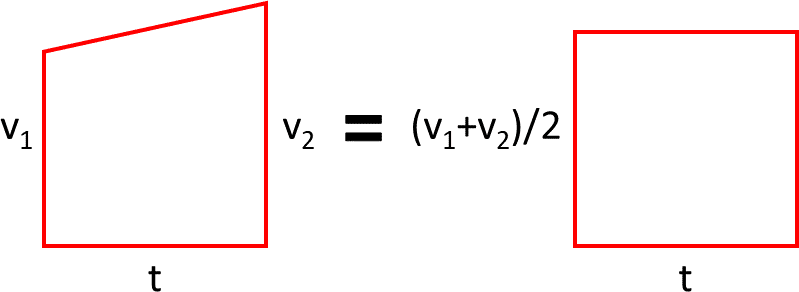
So now we can't just use the equation $v = s/t$ because that assumes that the velocity is constant, whereas here it has increased (steadily) from $v_1$ to $v_2$. Now without referring to Newton's equations of motion, it is clear that there exists a single constant velocity which is between $v_1$ and $v_2$ such that the distance travelled in the same duration is equal to the distance travelled after this acceleration. In other words, there is some rectangle with a height that is between $v_1$ and $v_2$ that should give the same answer. We usually call this height the average velocity and it is usually found by dividing the total distance travelled by the total duration of travelling. But here we don't have the distance travelled, only the initial and final velocity. So what is the average velocity of a uniformly increasing velocity?

The answer is the average height of the trapezium, which is $(v_1 + v_2)/2$. We can convince ourselves that this is the average height of the trapezium by sampling a number of points along the top side of the trapezium and finding what the average of the sample heights is. Let's take trapezium C in the brokendown graph above which is between time 20 and 25:

Of course since this is just a single case you might not be convinced yet; so let's do this algebraically using a variable amount of samples $n$:

$$ \hat{v} = \frac{\sum_{i \in 0...n-1}{(v_1 + \frac{i\times(v_2 - v_1)}{n-1})}}{n} \\ \hat{v} = \frac{\sum_{i \in 0...n-1}{v_1} + \sum_{i \in 0...n-1}{\frac{i\times(v_2 - v_1)}{n-1}}}{n} \\ \hat{v} = \frac{n v_1 + \frac{(v_2 - v_1)\times\sum_{i \in 0...n-1}{i}}{n-1}}{n} \\ \hat{v} = v_1 + \frac{(v_2 - v_1)\times\sum_{i \in 0...n-1}{i}}{n\times(n-1)} \\ \hat{v} = v_1 + \frac{(v_2 - v_1)\times\frac{n\times(n-1)}{2}}{n\times(n-1)} \\ \hat{v} = v_1 + \frac{v_2 - v_1}{2} \\ \hat{v} = v_1 + \frac{v_2}{2} - \frac{v_1}{2} \\ \hat{v} = \frac{v_2}{2} + \frac{v_1}{2} \\ \hat{v} = \frac{v_2 + v_1}{2} $$

Great! So now we know that given a trapezium of velocity-time graph, this is equivalent to a rectangle of the same width but with a height that is the average of the two sides:

We already know how to find the distance travelled by a rectangle shaped velocity-time graph so let's use it on the above rectangle: $s = (v2+v1)/2\times t$. It just so happens that this is also the area of the trapezium. So we can just skip all the above and just take the area of the trapezium to find the distance travelled.

All that's left is what is the distance travelled when the velocity is zero since it's just a flat line, but I'm sure you can guess what that is.

Friday, July 31, 2020

How to capture/redirect output in Python's print

The print function in Python v3 is one of the more sophisticated changes made from v2. You can tell it where to print by using the parameter 'file'. It can either print to the screen as usual or it can print into a text file for example. Here's how you make it print into a text file:

with open('x.txt', 'w', encoding='utf-8') as f:
    print('hello', file=f)

The 'file' parameter accepts a stream object and the print function basically just passes the string you give it to this stream object's 'write' method. In fact in the above example you could have written to the file without using print as follows:

with open('x.txt', 'w', encoding='utf-8') as f:
    f.write('hello')
    f.write('\n')
    f.flush()

So question is, what is the stream used by print when it prints to the screen? The print method's signature is defined as follows:

print(value, ..., sep=' ', end='\n', file=sys.stdout, flush=False)

So the answer is sys.stdout, which is a variable that points to the object sys.__stdout__. In fact you can make your own print function by using the sys.__stdout__ object as follows:

import sys

def my_print(line):
    sys.__stdout__.write(line)
    sys.__stdout__.write('\n')
    sys.__stdout__.flush()

my_print('hello')

Note that the output will appear in the command line terminal. Now we saw how the default file parameter of the print function is whatever sys.stdout is pointing to. This means that we can highjack this variable with our own stream so that default prints get redirected to our code instead of the screen. Here's how to make your own stream:

class MyStream(object):

    def write(self, text):
        pass

    def flush(self):
        pass

Just replace 'pass' in the write method with whatever you want and that is what will happen with the print string. Now normally you would do something like this:

print('hello', file=MyStream())

but if you're trying to capture the outputs of some library, like sklearn, then you don't have control over the library's print functions. Instead you can do this:

import sys

tmp = sys.stdout
sys.stdout = MyStream()

print('hello')

sys.stdout = tmp

First you hijack the stdout variable with your own stream and then after the prints you restore the stdout variable with the original stream. Now, you need to be careful with what happens inside your stream's write method because if there is another print in there then it will also call your stream's write method which will result in an infinite recursion loop. What you can do is temporarily restore the original stream whilst inside your stream, like this:

import sys

class MyStream(object):

    def write(self, text):
        tmp = sys.stdout
        sys.stdout = sys.__stdout__

        print('my', text)

        sys.stdout = tmp

    def flush(self):
        pass


tmp = sys.stdout
sys.stdout = MyStream()

print('hello')

sys.stdout = tmp

Now every time you print something, you'll get 'my' added to its front. Unfortunately the print function sends the '\n' at the end of the line in a separate call to the stream's write method, which means that you actually get two calls per print:

my hello
my


A simple solution is to just put an 'if' statement that checks if the text received is just a '\n' and ignore it if so:

import sys

class MyStream(object):

    def write(self, text):
        if text == '\n':
            return

        tmp = sys.stdout
        sys.stdout = sys.__stdout__

        print('my', text)

        sys.stdout = tmp

    def flush(self):
        pass


tmp = sys.stdout
sys.stdout = MyStream()

print('hello')

sys.stdout = tmp